Basis functions in quantum chemistry

Difference plane-wave and atomic-centered basis sets

One of the main approximations for electronic structure calculations is the introduction of a basis set used to describe the wavefunction. In the case of an incomplete basis we make an approximation of a molecular orbital. All electronic structure methods scale at least with \(M^4\) where M denotes the number of basis functions. Therefore, we want that our basis set is small and easy to evaluate in order to make computations fast.

Two main types exist:

• atomic-centered basis sets using gaussian or slater-type functions

• plane-wave basis sets using plane-wave basis functions.

A gaussian type atomic-centered orbital in polar or cartesian coordinates is commonly written as:

\[\begin{split} \begin{aligned} \chi_{\zeta, n, l, m}(r, \theta, \varphi) &=N Y_{l, m}(\theta, \varphi) r^{2 n-2-l} \mathrm{e}^{-\zeta r^{2}} \\ \chi_{\zeta, l_{x}, l_{y}, l_{z}}(x, y, z) &=N x^{l_{x}} y^{l_{y}} z^{l_{z}} \mathrm{e}^{-\zeta r^{2}} \end{aligned} \end{split}\]

The sum of \(l_x\), \(l_y\) and \(l_z\) determines the type or orbital.

A plane-wave orbital can be expressed as:

\[ \chi_{k}(\mathbf{r})=e^{i \mathbf{k} \cdot \mathbf{r}} \]

where \(k\) is the wave vector which is related to the energy \(E=\frac{1}{2} k^2\).

The allowed values for \(k\) are given by the unit cell translational vector \(t\) with \(k*t = 2\pi m\) where \(m\) a positive integer.

The role of \(k\) is similar to \(\zeta\) for gaussian type basis sets.

Plane-waves are well suited for describing delocalized slowly varying electron densities - e.g the valence bands in a metal.

The core electrons on the other hand are difficult to describe because they are strongly localized around the nuclei and contain many oscillations. They therefore require large \(k\) values. Therefore, in practice the nuclear charge is smeared and the core electrons approximated by a so called pseudopotential, which is fitted to reproduce on average the wavefunction of the core electrons and thus makes the calculation tractable.

For plane wave basis sets the number of plane waves depends on:

\[ N_{PW} = \frac{1}{2\pi^2} \Omega E_\text{cut}^{\frac{3}{2}} \]

where \(\Omega\) is the box volume.

An example of how the quality of the approximation changes with the core parameter (number of gaussians for atomic centered basis set vs. \(E_\text{cut}\) for plane wave basis set) is given here for the 3d-orbital in iron:

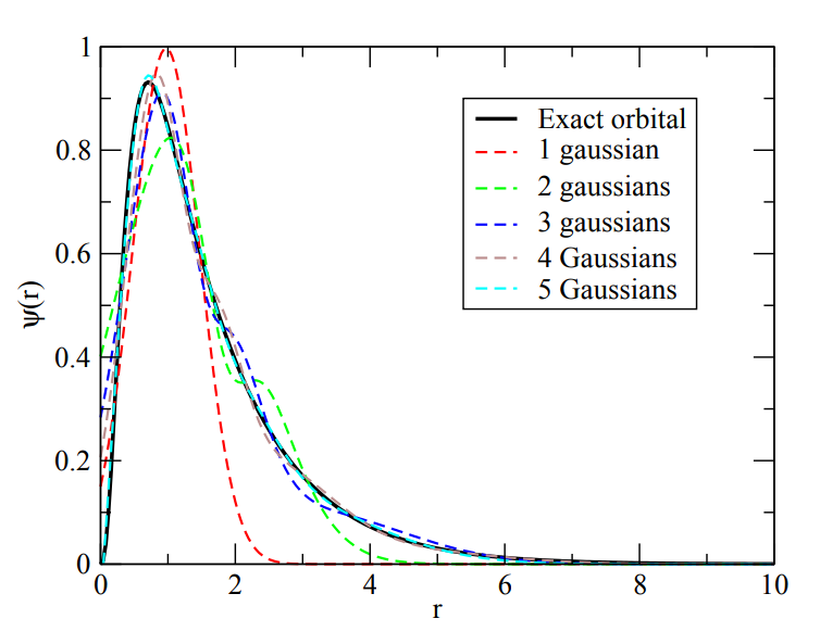
Fig. 1 Atomic centered basis functions to describe the 3d orbital in Fe. The quality increases with the number of gaussian used.

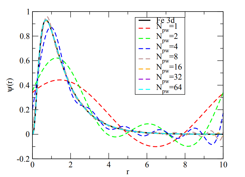
Fig. 2 Plane-wave basis functions to describe the 3d orbital in Fe. The quality increases with the cutoff energy and the box size.

Images taken from Archer Training Material

Comparison of atomic centered and plane wave basis sets

Atomic centered basis set	Plane wave basis set
➕ Consistent with chemical picture of molecules	➕ Consistent with chemical picture of solids
➕ Need few basis functions to well describe molecules	➖ Many basis functions required
➕ Inner electrons are not much more difficult than outer electrons	➖ Many oscillations for core electrons, need pseudopotential to describe core electrons
➕ Computation independent of empty volume of system	➖ Empty volume as expensive as the atoms in the calculation
➖ Non-orthogonal (if using Gaussians)	➕ Orthogonal
➖ No analytical derivatives (if using Slater type functions)
➖ Basis set superposition error	➕ No BSSE
➖ Many parameters to optimize/choose	➕ Single parameter to control quality (\(E_\text{cut}\)), to improve basis set improve cutoff
〰️ No periodicity	〰️ Periodic
〰️ Easily tunable (e.g use diffuse functions for anions)	〰️ All or nothing description (no spot prefered)
➖ Depends on atomic positions, forces are difficult to calculate	➕ Independent of atomic positons (no Pulay forces)

〰️ indicates properties that might be advantageous or disadvantageous depending on the system.