3.3. Geometry optimization of \(H_2O\)#
Until now we have used fixed positions of the nuclei. This means we created a molecule with specified x,y,z coordinates for each atom, passed it to psi4 and then we called psi4.energy(method/basisset). By running such a single point energy calculation we find the lowest energy solution for the Schroedinger equation at the current geometry.
Now, what if we do not know how our molecule looks like? E.g suppose the equilibrium bond length and the angle between the atoms of a triatomic molecule that you are looking at is unknown. How to find it?
The procedue to start from a starting geometry and arrive at an optimal geometry is called geometry optimization.
Consider the simple case of the hydrogen molecule, where the only parameter that can be optimised is the distance between the nuclei. The energy of every possible configuration is given by a two-dimensional potential energy surface (PES): Starting from an initial guess for the geometry, one may follow the curvature of the PES down to the minimal energy, which will correspond to the equilibrium geometry. In a practical geometry optimisation, this will be done in discrete steps of a certain size. At each iteration, the energy of the corresponding geometry is calculated in a SCF calculation.
Then, the gradient with respect to the nuclear coordinates is determined, and the nuclei are moved to a new position on the PES that lies in the direction of the steepest gradient. The geometry optimisation converges once the minimum is attained. In practice, this implies that the forces on the nuclei fall below a certain treshold.\
Larger systems will have more nuclear degrees of freedom than simple bimolecular species, and in these cases the PES becomes many-dimensional; each degree of freedom will correspond to one dimension. Geometry optimisations may not converge on very complex potential energy surfaces. If the program is fed with an input that resides in a region of the PES that has a difficult topology, the algorithm may not find a minimum, and it may be better to restart from a different initial geometry. Furthermore, a PES may exhibit multiple minima, and the geometry optimisation algorithm may only reach the next local minimum, but not neccessarily the global minimum.
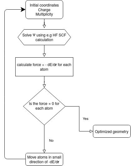
Fig. 3.1 Procedure of a geometry optimization.#
First again we again import the required modules:
import psi4
import pandas as pd
import numpy as np
import matplotlib.pyplot as plt

import plotly.graph_objects as go
import sys

sys.path.append("..")
from helpers import *
then we set the maximum ressources that can be used
psi4.set_memory('2 GB')
psi4.set_num_threads(4)
You will carry out a geometry optimisation on a bad guess for H\(_2\)O with an unrealistic H-O-H angle of 90\(^\circ\) and a O-H distance of 1.5Å. During the optimisation, Psi4 will move the positions of the atoms in the molecule, moving downhill on the potential energy surface, until it finds a minimum.
First, we define our suboptimal geometry. Again, we use a UHF reference.
r = 1.5
angle = 90

# Water Z-Matrix
h2o_suboptimal = psi4.geometry(f"""
O1
H2 1 {r}
H3 1 {r} 2 {angle}
""")

h2o_suboptimal_start = h2o_suboptimal.clone() # we store here the starting geometry for comparison
# setting the options to write out the xyz files of the optimization
psi4.set_options({'reference':'uhf'})
psi4.core.set_output_file(f'h2o-opt.log', False)
psi4.set_options({'write_trajectory':True})
psi4.set_options({'PRINT_TRAJECTORY_XYZ_FILE':True})
# start the geometry optimization
E,hist= psi4.optimize('hf/6-31G', molecule=h2o_suboptimal,return_history=True)
symbols = [h2o_suboptimal.symbol(i) for i in range(h2o_suboptimal.natom())]
bohr_to_ang = 0.52917721092
with open("geoms.xyz", "w") as f:
    for istep, coords in enumerate(hist['coordinates']):
        coords_ang = coords * bohr_to_ang
        f.write(f"{len(symbols)}  \n")
        f.write(f"Geometry for iteration {istep} \n")
        for sym, (x,y,z) in zip(symbols, coords_ang):
            f.write(f"{sym:2s} {x:15.10f} {y:15.10f} {z:15.10f}\n")
Let’s have a look at the initial and final conformation after the geometry optimization. We can use the drawXYZSideBySide helper funciton, which allows to show two molecules.
drawXYZSideBySide(h2o_suboptimal_start, h2o_suboptimal)
Lets have a look at the output file and see what is happening. Lets grep again the iter keyword as before and also check the convergence of the geometry optimization using Convergence Check.
!grep -A 1 -B 4 '@DF-UHF iter' h2o-opt.log
Exercise 6
Why are there multiple iterations of the SCF cycle?
!grep -A 10 'Convergence Check' h2o-opt.log
!grep 'Measures of convergence' h2o-opt.log | head -n 1
!grep 'Criteria marked as inactive' h2o-opt.log | head -n 1
!grep 'Step    Total Energy     Delta E' h2o-opt.log | head -n 1
!grep '~' h2o-opt.log
Exercise 7
Why does the optimization finish after several steps?
3.3.1. Visualization if the optimization procedure#
Now we want to visualize how the geometry is changed during the optimization procedure. Ler’s save the coordinates first:
optimized_geos = readXYZ('geoms.xyz')
coordinates =  read_coordinates('geoms.xyz')
We read in the coordinates as numpy arrays and as xyz files for visualization.
You can use the little helper function angle_distances to calculate the angle and O-H distances for all 8 optimization steps.
The first column of the array is the H-O-H angle, the second column and third column are the OH distances.
angle_dist = []
for coords in coordinates: # iterate over the list of coordinates, coords being a single point calculation result
    angle_dist.append(angle_distances(coords))

h2o_angles_dist = np.array(angle_dist[1:])
h2o_angles_dist
Let’s also extract the energies after each SCF cycle. We can use grep for this
geo_opt_energies = !grep -a '@DF-UHF Final Energy' h2o-opt.log
geo_opt_energies = [float(x.replace('  @DF-UHF Final Energy:   ',''))  for x in geo_opt_energies] # this is some formatting to get the values from the text file
geo_opt_energies
To help you visualizing the result, we have prepared a full potential energy surface of water at the HF/6-31G level. We will load it and the plot the path our geometry optimization takes based on the angle and the distance we extracted from the trajectory (for this we will use Plotly, a plotting library with 3D capabilities which we imported at the beginning).
The potential energy function that is plotted was calculated by performing single point energy calculations for water in 40 steps ffor all angles between 20 and 170° and distances between 0.6 and 2 Å.
# load in files for PES
PES_water = np.load('PES_water/water-hf-6-31G-energies.npy')
PES_r = np.load('PES_water/water-hf-6-31G-distances.npy')
PES_angle = np.load('PES_water/water-hf-6-31G-angle.npy')
# this sets up the plotting widget
fig = go.Figure(data=[go.Surface(z=PES_water,
                                 x=PES_r,
                                 y=PES_angle,
                                 colorscale='RdBu',
                                 reversescale=True,
                                 hoverinfo='none',
                                 name='Full PES',
                                 contours=go.surface.Contours(
                                    x=go.surface.contours.X(highlight=False),
                                    y=go.surface.contours.Y(highlight=False),
                                    z=go.surface.contours.Z(highlight=False),
                                )
                                )
                     ])
# here we plot our geometry optimization results
# change the z, x, y options if you plot multiple lines, you can also change the colors
fig.add_scatter3d(z=geo_opt_energies, x=h2o_angles_dist[:,1], y=h2o_angles_dist[:,0],mode='markers+lines', marker=dict(size=3, color='orange', opacity=1),
                   line=dict(color='darkorange',width=2),
                   name="Geometry Optimization"
                 )

# this is comesmetics to add labeles etc.
fig.update_layout(title='Water Potential Energy Surface', autosize=False,
                  template='simple_white',
                  width=900, height=900,
                  scene = dict(
                      xaxis_title="O-H [A]",
                      yaxis_title="Angle H-O-H",
                      zaxis_title='Energy [a.u]',
                      xaxis_showspikes=False,
                      yaxis_showspikes=False),
                   margin=dict(l=65, r=50, b=65, t=90))
# to display the figure
fig.show()
We can also look at the molecules using the command below:
drawXYZGeomSlider(optimized_geos)
Exercise 8
Try to start from two (or more!) different suboptimal geometries of water and include the plots of the potential energy surface in the report, together with a screenshot of the starting and final geometry and/or the values of the O-H bond and H-O-H angle.
What do the points on the orange curve correspond to? Connect them to the flowchart at the beginning of this exercise?