5.1. Theory

5.1.1. Classical Molecular Dynamics

The extensive computational demand of electronic structure elucidation implies that an exact (fully quantum mechanical) description and time-propagation of even modestly sized molecular systems is in practice impossible. Although systems that comprise about \(10^3\) atoms are nowadays routinely described using approximate quantum mechanical (such as state-of-the-art Kohn-Sham Density Functional Theory) or semi-empirical methods, the computational demand of explicitly treating electrons in even larger systems such as biomolecules (\(10^5\) atoms and more) becomes untractable all too quickly.

Fortunately, for such systems it is frequently sufficient to use a classical approximation to accurately reproduce supramolecular properties, such as the folding of a protein or the structure of a liquid. Classical approximations typically scale better with system size, and they therefore allow both for large systems and long simulation times to be taken into account. Here, atoms are treated as effective point charges with mass, instead of nuclei with explicit electrons. The classical approach makes use of a parameterised force field (or classical potential energy function), which is an approximation of the quantum-mechanical potential energy surface due to the electronic and nuclear potential, as a function of nuclear position. Such classical force fields typically work well under the following assumptions:

1. The Born-Oppenheimer approximation is valid.

2. The electronic structure is not of interest.

3. The temperature is modest.

4. There is no bond breaking or forming.

5. Electrons are highly localised.

5.1.2. Classical Approximation: Basic Features

In the classical approximation, one describes positions and momenta of all the atomic nuclei:

(5.1)\[\begin{split} \begin{aligned} \mathbf{r}^N &= \{x^1, y^1, z^1, \ldots,x^N, y^N, z^N\} \\ \mathbf{p}^N &= \{p_{x1}, p_{y1}, p_{z1}, \ldots,p_{xN}, p_{yN}, p_{zN}\}, \end{aligned} \end{split}\]

where each position and all momenta are known simultaneously. One microstate is then characterised by a set of the \(3N\) positions \(\{\mathbf{r}^N\}\) and \(3N\) momenta \(\{\mathbf{p}^N\}\) for a total of 6N degrees of freedom, such that the notation \(\{\mathbf{p}^N_m, \mathbf{r}^N_m\}\) defines a particular microstate \(m\). For any microstate, one can calculate the total energy as a sum of the kinetic \(T(\{\mathbf{p}^N\})\) and potential \(V(\{\mathbf{r}^N\})\) terms. The Hamiltonian of a classical system then becomes:

(5.2)\[ \mathbf{H}(\{\mathbf{p}^N\}, \{\mathbf{r}^N\}) = \mathbf{T}(\{\mathbf{p}^N\}) + \mathbf{V}(\{\mathbf{r}^N\}), \]

where the kinetic term is simply:

(5.3)\[ \mathbf{T}(\{\mathbf{p}^N\}) = \sum_i^N \frac{|\mathbf{p_i}|^2}{2m_i}. \]

Interactions between atoms are then described by a potential energy function \(\mathbf{V}(\{\mathbf{r}^N\})\) that depends solely on the positions of all atoms \(\{\mathbf{r}^N\}\). A key part of describing time evolution of a molecular system classically is then the definition of the potential energy function \(\mathbf{V}(\{\mathbf{r}^N\})\). In fact, the functional form of \(\mathbf{V}(\{\mathbf{r}^N\})\) is often chosen by examining the various modes by which atoms interact according to a quantum mechanical treatment of the molecular system and patching simple, often first-order theoretical expressions for these modes together. These modes can also be fitted to experimental (and/or quantum mechanical calculations of) model compounds such that the force field reproduces selected properties of a database of representative test structures.

\(\mathbf{V}(\mathbf{r}^N)\) can be mainly decomposed into the following components:

(5.4)\[ \mathbf{V}(\{\mathbf{r}^N\}) =\mathbf{V}_{bonded}(\{\mathbf{r}^N\}) + \mathbf{V}_{non-bonded}(\{\mathbf{r}^N\}), \]

where \(\mathbf{V}_{bonded}(\{\mathbf{r}^N\})\) and \(\mathbf{V}_{non-bonded}(\{\mathbf{r}^N\})\) correspond to intermolecular and intramolecular potentials respectively. Intramolecular interactions typically include bond stretching, bond angle bending and bond torsional modes, while intermolecular interactions include dispersion and coulombic potentials. These are discussed in more detail below.

5.1.2.1. Intramolecular Interactions

Intramolecular interactions occur through bonds between atoms, the three most well known being bond stretching (vibration), bond angle bending and bond torsional modes. These are illustrated in Fig. 5.1

Fig. 5.1 Depiction of the 2, 3, and 4-centre intramolecular forces.

5.1.2.1.1. Bond Stretching

An accurate description of bond stretching that well-describes the intramolecular behaviour is the empirical Morse potential:

(5.5)\[ V_B(d) = D_e[1-e^{-a(d-d_0)}]^2, \]

where \(d\) is the length of the bond, \(a\) is a constant, \(d_0\) is the equilibrium bond length, and \(D_e\) is the well-depth minimum. Typically this form is not used, as it requires three parameters per bond and is somewhat expensive to compute in simulation due to the exponential. Since the energy scales of bond stretching are relatively high, bonds rarely deviate significantly from the equilibrium bond length, thus one can use a second-order Taylor expansion around the energy minimum:

(5.6)\[ V_B(d) = \alpha(d-d_0)^2, \]

where \(\alpha\) is a constant. This form treats bond vibrations as harmonic oscillations, and thus atoms cannot be dissociated. Fig. 5.2 provides a depiction of both the Morse potential and the corresponding harmonic approximation.

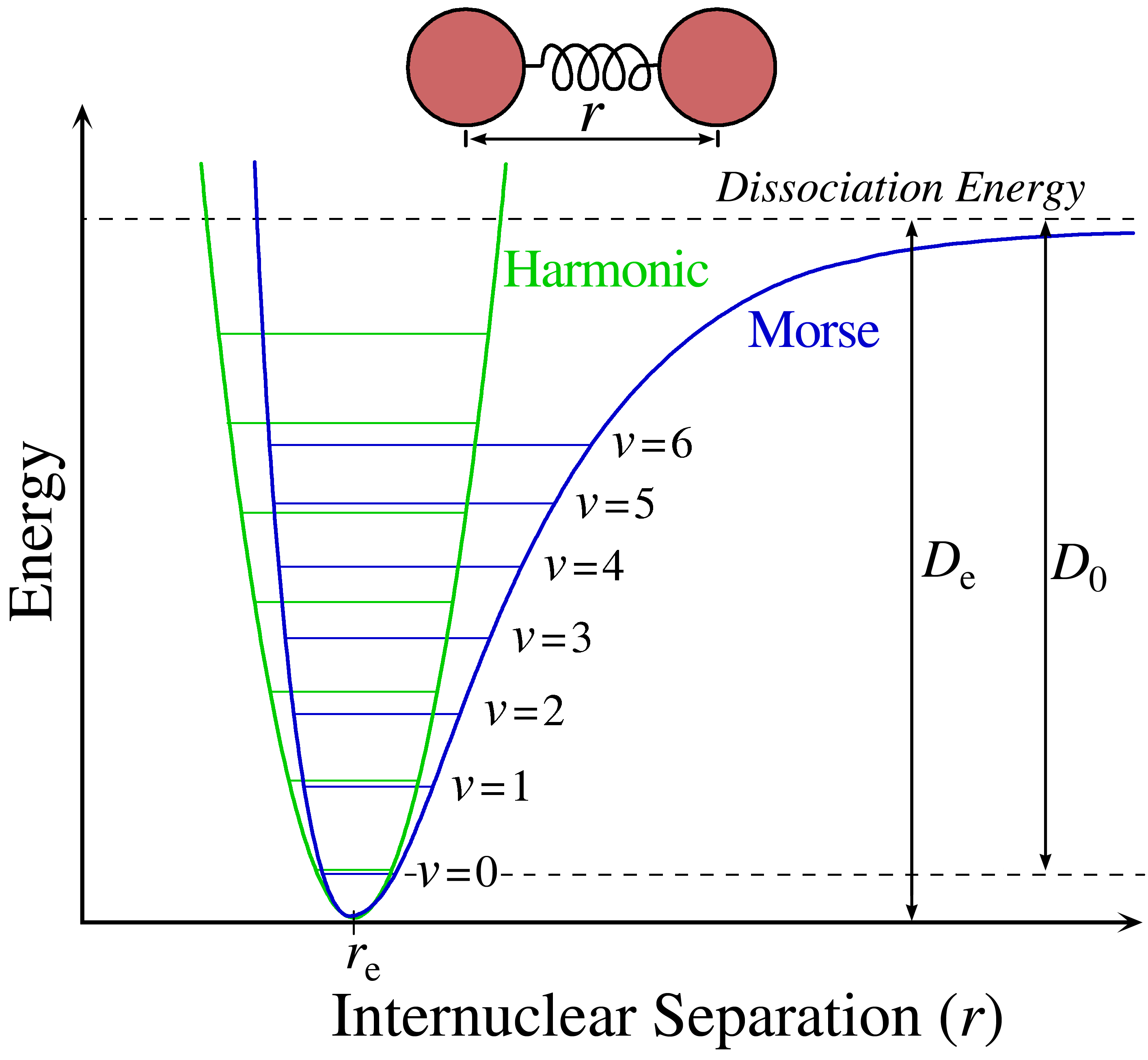
Fig. 5.2 Depiction of a Morse and harmonic potential used to approximate chemical bonds. CC by SA 3.0 Somoza

5.1.2.2. Bond Angle Bending

This term accounts for deviations from the preferred hybridisation geometry (e.g sp\(^3\)). Again, a common form is the second-order Taylor expansion about the energy minimum:

(5.7)\[ V_A(\theta) = b(\theta-\theta_0)^2, \]

where \(\theta\) is the bond angle between three atoms, \(b\) is a constant and \(\theta_0\) is the equilibrium bond angle.

5.1.2.3. Bond Torsions

These interactions occur among four atoms and account for rotational energies along bonds. Unlike the previous terms, torsional modes are “soft” such that energies are often not so high as to only allow small deviations from an equilibrium structure. Torsional modes are frequently modeled with the following expression:

(5.8)\[ V_T(\phi)= \sum_{n=0}^N k_n[1 + cos(n\phi - \delta)], \]

where \(\phi\) is the torsional angle, \(n\) is the periodicity and \(k_n\) is the rotational energy barrier, and \(\gamma\) is an additional dihedral-dependent parameter which models the offset of the minima. A depiction of \(V_T(\omega)\) is provided in Fig. 5.3

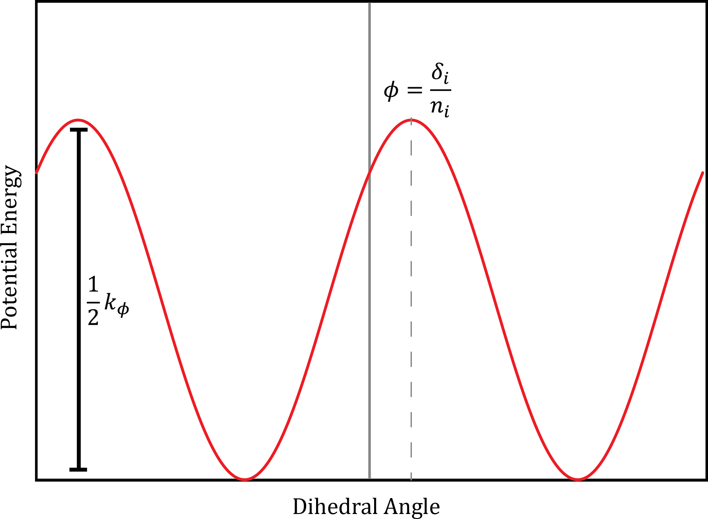
Fig. 5.3 The representation of the potential energy of a torsional angle rotation using a cosine representation. CC by SA cnrowley

5.1.3. Intermolecular Interactions

Intermolecular interactions apply to any atoms that are not bonded, either within the same molecule or between different molecules.

These interactions are described using a pairwise decomposition of the energy. Formally one can decompose the potential energy function into interactions involving single atoms, pairs of atoms, triplets of atoms and so forth:

(5.9)\[ \mathbf{V}(\{\mathbf{r}^N\}) = \sum_{i=1}^N \mathbf{v}_1(\mathbf{r}_i) + \sum_{i=1}\sum_{j=i+1} \mathbf{v}_2(\mathbf{r}_{ij}) + \sum_{i=1}\sum_{j=i+1}\sum_{k=j+1}\mathbf{v}_3(\mathbf{r}_{ij}, \mathbf{r}_{ik}, \mathbf{r}_{jk}) + \dots. \]

It is convenient to truncate this expansion beyond pairwise interactions as the computational expense of adding additional terms scales as \(O(N^k)\), where \(k\) is the number of bodies interacting. This truncation is performed at the expense of certain polarization effects which can lead to subtle deviations away from experimental results. The resulting effective pair potential is given by:

(5.10)\[ \mathbf{V}(\{\mathbf{r}^N\}) = \sum_{i=1}^N \mathbf{v}_1(\mathbf{r}_i) + \sum_{i=1}\sum_{j=i+1} \mathbf{v}_{eff}(\mathbf{r}_{ij}). \]

5.1.3.1. Electrostatics

Interactions between charges (partial or formal) are modeled using Coulomb’s law:

(5.11)\[ \mathbf{V}_{c}(\mathbf{r}_{ij}) = \frac{q_i q_j}{4 \pi \epsilon_0 \mathbf{r}_{ij}}, \]

for which the atoms \(i\) and \(j\) are separated by distance \(\mathbf{r}_{ij}\). The partial charges are given by \(q_i\) and \(q_j\) while \(\epsilon_0\) denotes the free space permittivity.

5.1.3.2. London Dispersion Forces

Correlations between instantaneous electron densities surrounding two atoms gives rise to an attractive potential:

\[ \mathbf{V}_{ld}(\mathbf{r}_{ij}) \propto \mathbf{r}_{ij}^{-6} \]

and is a component of the Van der Waals force, which contains other forces including dipole-dipole (Keesom force), permanent dipole-induced dipole (Debye force) and London dispersion forces. A depiction of London dispersion and Coulombic forces can be seen in Fig. 5.4

Fig. 5.4 Depiction of London dispersion and Coulombic forces.

5.1.3.3. Excluded Volume Repulsion

When two atoms approach and their electron densities overlap, they experience a steep increase in energy and a corresponding strong repulsion. This occurs due to the Pauli principle: two electrons are forbidden to have the same quantum number. At moderate inter-nuclear distances, this potential has the approximate form:

(5.12)\[ \mathbf{V}_{evr}(\mathbf{r}_{ij}) \propto e^{-c \mathbf{r}_{ij}}, \]

where \(c\) is a constant. To alleviate computational complexity this can be successfully modeled by a simple power law that is much more convenient to compute:

(5.13)\[ \mathbf{V}_{evr}(\mathbf{r}_{ij}) \propto \mathbf{r}_{ij}^{-m}, \]

where \(m\) is greater than 6.

5.1.3.4. Lennard-Jones Potential

An effective method to model both the excluded volume and London dispersion forces is to combine them into a single expression, which Lennard-Jones proposed in the following pairwise interaction:

(5.14)\[ \mathbf{V}(\mathbf{r}_{ij}) = 4 \epsilon_{ij} \left[ \left( \frac{\mathbf{r}_{ij}}{\sigma}\right)^{-12} - \left( \frac{\mathbf{r}_{ij}}{\sigma}\right)^{-6} \right] \]

where \(\epsilon\) and \(\sigma\) are atom-dependent constants. The factor of 12 is used for the repulsive term simply because it is convenient to square the attractive \(\mathbf{r}_{ij}^{-6}\) term.

5.1.4. The Atomic Force Field

A bare-minimum force field can now be constructed as a simple addition of individual contributions to the approximation of the potential energy surface:

(5.15)\[\begin{split} \begin{gathered} \mathbf{V}(\{\mathbf{r}^N\}) = \sum_{\text{bonds}, i}\alpha_i(d_i - d_{i,0})^2 + \sum_{\text{angles}, j}\beta_j(\theta_j - \theta_{j,0})^2+ \sum_{\text{torsions}, k} \left[ \sum_{n=0}^N k_n[1 + cos(n\phi - \delta)]\right] \\ + \sum_i \sum_{j < i} \frac{q_i q_j}{4 \pi \epsilon_0 \mathbf{r}_{ij} } + 4\epsilon_{ij} \left[ \left(\frac{\mathbf{r}_{ij}}{\sigma_{ij}}\right)^{-12} - \left(\frac{\mathbf{r}_{ij}}{\sigma_{ij}}\right)^{-6} \right]. \end{gathered} \end{split}\]

5.1.4.1. Force Field Parameterisation and Transferability

The minimal force field in section Section 5.1.4 contains a large number of parameters:

(5.16)\[ \alpha_i, d_{i,0},\beta_j, \theta_{j, 0}, c_{k,n}, \gamma_k, q_{i,j}, \epsilon_{ij}, \sigma_{ij}, \delta, k_n \]

which must be chosen, depending on the kind of atoms involved and their chemical environment (e.g an oxygen-bound carbon behaves differently to a nitrogen-bound carbon), for every single type of bond, angle, torsion, partial charge and repulsive/dispersive interaction. In fact, all modern force fields typically contain more functions than the minimal and hence this results in a huge set of adjustable parameters that define a particular force field. Classical force fields are an area of active research, and are continually and rigorously developed and improved by a number of different research groups. Values for these parameters are typically taken from a combination of electronic structure calculations of small model molecules, and also experimental data. The inclusion of experimental data tends to improve accuracy because it fits bulk phases rather than the very small systems ab initio simulations can treat and as a result, the majority of force fields are semi-empirical.

5.1.5. Sampling specific ensembles

When running a Molecular dynamics simulation, we often want to sample from a specific ensemble. In a standard MD run as implemented in the toy example in Exercise 4 we sample in the microcanonical ensemble - \(NVE\). \(N\) is constant as we do not add or remove particles during the simulation, \(V\) is constant as the size of the box does not change, and \(E\) is constant as we use an integrator that conserves energy. In the NVE ensemble we will get the truly correct dynamics of the system. If we want to compare our simulation to experimental values then we however need to use either the canonical ensemble - \(NVT\) or the isothermal-isobaric ensemble \(NpT\).

In order to run in the NVT ensemble, we can use our NVE simulation code, and adjust the total energy such that the average temperature is equal to the one we want to simulate it. We can adjust the total energy easily by changing the momenta. The routine of doing this is called thermostat or barostat for the pressure.

5.1.5.1. Velocity rescaling

Clearly the simplest form of a thermostat is to rescale all velocities after each update so that their distribution matches the target temperature \(T_0\). This will however not produce realistic dynamics as it does not allow fluctations in the temperature which are present e.g in the canonical ensemble. In the NVT ensemble we expect that on average we sample at the \(T_0\) but the instantenous temperature \(T\) should vary. (See derivation p.141 in Frenkel & Smit).

(5.17)\[ v_i = \sqrt{\frac{T_0}{T}} v_i \]

5.1.5.2. Berendsen thermostat

An improvement of the rescaling algorithm for temperature control is the Berendsen thermostat. Sometimes, also called proportional thermostat. The Berendsen thermostat tries to correct the deviations of the instantenous temperature \(T\) from our target temperature \(T_0\) by multiplying the velocities by a factor \(\lambda\) in order to move the system dynamics towards the one corresponding to \( T_0\). This method does therefore allow temperature fluctuations.

In the Berendsen thermostat we set the rate of change of the temperature to

(5.18)\[ \frac{dT(t)}{dt}= \frac{1}{\tau} (T_0 -T) \]

the coupling parameter thus is:

(5.19)\[ \lambda^2 = 1 + \frac{dt}{\tau} * (\frac{T_0}{T} -1) \]

This thermostat however still does not sample the canonical ensemble and therefore should not be used in production simulations. The Berendsen thermostat samples the isokinetic ensemble. In particular this can lead to the so called flying ice cube effect, where high frequency modes such as vibrations are all drained into low frequency modes such as translation. While the kinetic energy is conserved this violates the equipartition of energy and is clearly an algorithmic artefact.

Standard MD simulation programs such as Gromacs use a modification of this thermostat called the Bussi-Donadio-Parrinello thermostat (v-rescale in Gromacs). Here, the velocities are not rescaled to match the target temperature but the velocities are scaled to a kinetic energy that is stochastically chosen from the kinetic energy distribution dictated by the canonical ensemble.

5.1.5.3. Andersen thermostat

An alternative approach to control temperature is to mimic collisions with a heat bath. This can be easily implemented by picking random atoms and drawing a new velocity from the Maxwell-Boltzman temperature at the target temperature Fig. 5.5. In between collisions the dynamics is according to NVE but due to the collisions samples from the canonical ensemble.

The strength of coupling to the heat bath is determined by \(\nu\) which has a similar function to \(\tau\) in the Berendsen thermostat. While the Andersen thermostat samples the \(NVT\) ensemble rigorously it will clearly disturb the natural dynamics of the system due to the abrupt nature of the collisions.

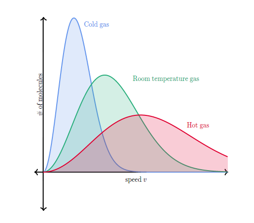
Fig. 5.5 Maxwell Boltzmann distribution for three different temperatures. Figure CC by SA Khan Academy

5.1.5.4. Nose-Hoover thermostat

Another popular thermostat is the Nose-Hoover thermostat. Here, an extended Lagrangian formalism is used, i.e no random velocities are used. Instead one uses a friction factor to control particle velocities. This dimensionless factor belongs to a an additional degree of freedom which has mass \(Q\).

The new equations of motions are

(5.20)\[ \frac{\text{d}v(t)}{\text{d}t} = \frac{\mathrm{F}(t)}{m} - \zeta \mathrm{v}(t) \]

with \(\zeta\) the thermodynamic friction coefficient as

(5.21)\[ \frac{\mathrm{d} \zeta(t)}{\mathrm{d} t}=\frac{1}{Q}\left[\sum m \mathbf{v}(t)^{2}-(N_{DOF}+1) k_{B} T\right] \]

\(Q\) has dimension of \(\text{energy} \times (time)^2\) and controls the temperature fluctation.

The main advantage of the Nose-Hoover thermostat is that the additional degree of freedom is deterministic and time-reversible. However, for systems with very stiff degrees of freedom (i.e when a part of the system does not strongly interact with the rest of the system) use of the Nose-Hoover thermostat can lead to non-ergodicity. Here, a newer implementation of so called Nose-Hoover chains should be used. Here, we simply use a chain of Nose-Hoover thermostats that control the temperature and this leads to correct ergodic sampling.

In practice, for most simulations one should use the Berendsen Thermostat with the stochastic term by Bussi, Donadio and Parrinello or the Nose-Hoover Chain thermostat.

5.1.6. Initialization

In order to run a sucessful simulation to sample a property of interest it is important to start with a correct structure.

After having obtained an initial geometry of the system we want to simulate the question remains on how to initialize our system to avoid lengthy equilibration. Simply setting the velocity of each particle to \(0\) as we did in the last exercise clearly is not very realistic and will not converge easily to our target temperature.

As running a molecular dynamics simulation is equivalent to computationally sampling from a thermodynamic ensemble it is clearly more appropriate to start with a configuration that has close resemblance to a configuration derived from the ensemble we want to simulate in e.g at fixed number of particles \(N\), fixed volume \(V\) and finite temperature \(T_0\). This means that the velocities of the particles should resemble the distribution of velocities at the target temperature to be a realistic structure from that ensemble.

We know that in equilibrium the distribution of velocities is the Maxwell Boltzmann distribution Fig. 5.5.

To initialize our MD simulation, we therefore choose random velocities from a gaussian distribution with \(\mu=0\) and variance corresponding to the target temperature in order to emulate the Maxwell Boltzmann distribution. These starting velocites will quickly be randomized and our thermostat will take care of ensuring that we simulate in the target ensemble (if simulating in \(NVT\) or \(NpT\)).

From, the equipartition theorem we know that each quadratic degree of freedom \(<\vec{v_x}>\), \(<\vec{v_y}>\), \(<\vec{v_z}>\) will contribute \(\frac{1}{2} K_B T\) to the kinetic energy which we can use to set the variance of the velocity distribution, where the following equality holds:

(5.22)\[ E_{kin,x} = \frac{1}{2} K_B T = \frac{1}{2} m v_x^2 \]

5.1.7. Pair Radial Distribution Functions \(g(r)\)

Radial distribution (Pair correlation) functions are of fundamental importance in thermodynamics, since macroscopic thermodynamic properties can usually be calculated directly from \(g(r)\). In short, they simply describe how probability density varies as a function of distance from a reference particle.

The partition function \(Z\) can be evaluated, in principle, by carrying out the integrations for a substance with a known potential function. However, this task is very difficult due to the very large number of molecules involved in real systems. A more convenient formulation is based on the concept of distribution functions. The probability \(P(N)\) of finding molecule 1 in volume element \(\mathrm{d}\mathbf{r}_1\) at \(\mathbf{r}_1\), molecule 2 in volume element \(\mathrm{d}\mathbf{r}_2\) at \(\mathbf{r}_2\), \(\ldots\), and molecule N in volume element \(\mathrm{d}\mathbf{r}_N\) at \(\mathbf{r}_N\) is given by:

(5.23)\[ P(N)\mathrm{d}\mathbf{r}_1 \ldots \mathrm{d}\mathbf{r}_N = \frac{1}{Z_c(N,V,T)}e^{-\frac{U_N}{k_BT}}\mathrm{d}\mathbf{r}_1 \ldots \mathrm{d}\mathbf{r}_N, \]

where \(U_N(\mathbf{r}_1,\dots,\mathbf{r}_N)\) is the potential energy due to the interaction between particles and \(Z_c(N,V,T)\) is the configurational integral,

(5.24)\[ Z_c(N, V, T) = \int{\ldots}\int{e^{-\frac{U_N}{k_BT}}\mathrm{d}\mathbf{r}_1\ldots \mathrm{d}\mathbf{r}_N}, \]

taken over all possible combinations of atomic particle positions. Generally the total number of particles is massive enough such that \(P(N)\) is not particularly useful. It is more informative to consider the relative position of two molecules irrespective of the location of other molecules in the system. Integrating equation (5.23) over all coordinates except those pertaining to the two molecules of interest, one obtains the definition of the second-order disitribution function \(p^{(2)}(\mathbf{r}_1, \mathbf{r}_2)\), which gives the probability of finding molecule 1 in volume element \(\mathrm{d}\mathbf{r}_1\) at \(\mathbf{r}_1\) and molecule 2 in volume element \(\mathrm{d}\mathbf{r}_2\) at \(\mathbf{r}_2\):

(5.25)\[ p^{(2)}_{ij}(\mathbf{r}_1, \mathbf{r}_2) = N_i(N_j - \delta_{ij}) \frac{1}{Z_c (N, V, T)}\int{\ldots}\int{e^{-\frac{U_N}{k_BT}}} \mathrm{d}\mathbf{r}_3\ldots \mathrm{d}\mathbf{r}_N, \]

where \(\delta_{ij}\) is the Kronecker delta. Note that \(p^{(2)}(\mathbf{r}_1, \mathbf{r}_2)\) depends on temperature, density and composition additionally to \(\mathbf{r}_1\) and \(\mathbf{r}_2\). For molecules which interact with radially symmetric potential functions \(p^{(2)}(\mathbf{r}_1, \mathbf{r}_2)\), in the fluid state, depends only on the distance between centres of masses \(r_{12}=|\mathbf{r}_1 - \mathbf{r}_2|\). In the limit of ideal gas (\(\frac{U}{k_BT} \rightarrow 0\)), the distribution function \(p^{(2)}(\mathbf{r}_1, \mathbf{r}_2)\) approaches the value \(N_i(N_j - \delta_{ij}) / V^2\). This suggests defining the pair radial distribution function, \(g^{(2)}_{ij}(r)\) by:

(5.26)\[ g^{(2)}_{ij}(r) = \frac{p^{(2)}_{ij}(r) V^2}{(N_i N_J)}, \]

which approaches \(1 - \delta_{ij}/N_j\) in the above limit. Combining equations (5.25) and (5.26) gives:

\[ g^{(2)}_{ij}(r) = V^2\left(1 - \frac{\delta_{ij}}{N_j}\right)\frac{1}{Z_c (N, V, T)}\int{\ldots}\int{e^{\frac{-U_N}{k_BT}}}\mathrm{d}\mathbf{r}_3\ldots \mathrm{d}\mathbf{r}_N, \]

which is the second-order correlation function (pair radial distribution function). If the system consists of spherically symmetric particles \(g^{(2)}_{ij}\) depends only on the relative distance between them \(r_{ij} = r_j - r_i\). Taking particle 0 as fixed at the origin of the coordinate system, \(\rho g(r)\mathrm{d}r = \mathrm{d}n(r)\) is the number of particles (among the remaining \(N-1\)) to be found in the volume \(\mathrm{d}r\) around the position \(r\). These particles can then be formally counted as:

(5.27)\[ \mathrm{d}n(r) = \left<\sum_{i \neq 0}\delta (r - r_i)\right> \mathrm{d}r \]

where \(\langle\dots\rangle\) denotes the ensemble average, yielding:

(5.28)\[ g(r) = \frac{1}{\rho}\left<\sum_{i \neq 0}\delta(r - r_i)\right> = V\frac{N-1}{N}\left<\delta(r - r_1)\right> \]

where the second equality requires the equivalence of particles \(1,\dots, N - 1\).