2.1. Statistical Thermodynamics and the Boltzmann Distribution

This set of exercises brings together the theory of statistical mechanics with a practical example, the harmonic oscillator. After a brief (re)introduction to statistical mechanics, you will write a code that computes the probability distribution of the energy of a system using Boltzmann statistics.

2.1.1. Background

2.1.1.1. Statistical Thermodynamics

The average behaviour of a macroscopic system, the state of which is uncertain, can be studied using probability theory (statistical mechanics). However, such a probabilistic description cannot make thermodynamic properties accessible, unless a link between thermodynamic (free energy, pressure, entropy) and mechanical (position, momenta) properties can be introduced on the microscopic scale. Statistical thermodynamics (or equilibrium statistical mechanics) is concerned with the description of classical thermodynamics from a microscopic picture in terms of the particles that constitute the thermodynamical system. Statistical thermodynamics thus provide a link between the system’s microscopic properties and its macroscopic behaviour. The following constitutes a brief summary of the most important concepts in statistical mechanics (phase space, entropy as a phase space volume, partition functions). The discussion starts from the classical description of the microcanonical ensemble and is then extended onto the canonical and grandcanonical ensemble, with a link between quantum mechanics and the canonical ensemble being provided at the end of this chapter

Any system that consists of \(N\) particles can be characterised in terms of a 6N-dimensional set of variables: 3N coordinates \(\mathbf{q} = \left\{\mathbf{q}_1,\dots,\mathbf{q}_N\right\}\) and 3N momenta \(\mathbf{p} = \left\{\mathbf{p}_1,\dots,\mathbf{p}_N\right\}\). At every instant, the system is described by the values of \(\mathbf{p}\) and \(\mathbf{q}\) within a 6N-dimensional space, the phase space \(\Gamma = \left(\mathbf{p},\mathbf{q}\right)\). The point in phase space that characterises its current state identifies a point referred to as the representative point. The system i.e. its representative point will evolve within phase space according to its Hamiltonian:

(2.1)\[ \begin{align} H = \sum_{i=1}^N \left[\frac{\mathbf{p}_i^2}{2m_i} + U\left(\mathbf{q}_1,\dots,\mathbf{q}_N\right) \right]. \end{align} \]

Note that in the classical limit, the Hamiltonian is not an operator, but a sum over kinetic and potential energy terms. The evolution of the system in phase space is governed by Hamilton’s equations of motion:

(2.2)\[\begin{split} \begin{align} \frac{\mathrm{d}\mathbf{p}_i}{\mathrm{d}t} &= -\frac{\partial{H}}{\partial{\mathbf{q}_i}}\\ \frac{\mathrm{d}\mathbf{q}_i}{\mathrm{d}t} &= \frac{\partial{H}}{\partial{\mathbf{p}_i}}. \end{align} \end{split}\]

As is evident from (2.2), this formulation is an equivalent of Newtonian mechanics. Given a representative point, the evolution of the system in phase space is thus fully determined by Hamilton’s equations of motion. For an isolated system of constant particle number \(N\), constant volume \(V\) and constant energy \(E\), the trajectory of the system will lie on a hypersurface defined by:

(2.3)\[ \begin{align} H = E = \text{const.} \end{align} \]

Such a constant-\(NVE\) system of particles is described by a statistical ensemble referred to as the microcanonical ensemble. In the microcanonical ensemble, a system will move on the 6N dimensional hypersurface spanned by coordinates and momenta that lead to the same total energy \(E\).

Each of the possible representative points \(\mathbf{p},\mathbf{q}\) that give rise to the same energy \(E\) correspond to one microstate of the system. In general, for a thermodynamic state that is characterised by a set of extensive variables \(\left\{X_0,\dots,X_r\right\}\), the \(\left\{X_i\right\}\) will be a function over microscopic states \(\left\{\mathbf{p},\mathbf{q}\right\}\), such that \(X(\mathbf{r},\mathbf{q}) = X(\Gamma)\). The region of phase space that is accessible to the system \(X(\mathbf{p},\mathbf{q})\) is thus determined and limited by the values of \(X\). Such an `accessible region’ in phase space is (within the error of the variables \(X\)) denoted by \(W(E)\), with the corresponding volume element being \(|W(E)|\). According to the fundamental postulate of statistical mechanics, since every microstate has the same energy, the system is equally likely to be found in any of its microstates. In terms of the volume element in phase space, the probability to find the system in one of its microstates is:

(2.4)\[ \begin{align} P(E) = \frac{1}{|W(E)|}. \end{align} \]

Based on \(W(E)\), any thermodynamical property and observable is now accessible as a phase-space or ensemble average. For a microcanonical ensemble, the expectation value of an observable \(O\) is simply:

(2.5)\[ \begin{align} \left< O \right > = \int_{\Gamma \in W(E)} \frac{1}{|W(E)|} O(\Gamma) \mathrm{d}\Gamma , \end{align} \]

where the integration is over the 6N variables within the phase space volume elements \(d\Gamma\) that are contained in \(W(E)\). The above equation is nothing but the probability density of the system to be in a macroscopic state with the property \(O\) (recall the general form of a probability density).

Macroscopic observables are therefore linked to microscopic quantities using simple tools of statistics.

The Hamiltonian quantifies the kinetic and potential energy of the system, but the concept of entropy has been absent from the discussion so far. According to Boltzmann’s fundamental postulate of statistical thermodynamics, the entropy of a system is linked to the accessible volume \(W(E)\) in phase space, i.e. the entropy of a system in state \(X(\Gamma)\) is related to the volume accessible to \(X\):

(2.6)\[ \begin{align} S = k_B \ln |W(E)|, \end{align} \]

where \(S\) is the entropy as introduced for macroscopic systems, and \(k_B\) is Boltzmann’s constant.

Thus, a link between thermodynamic quantities and the system’s microscopic states is established, allowing for the prediction of any thermodynamic observable.

However, the 6N dimensionality of the problem restricts the analytic expressions of the above equations to small model systems; thermodynamic properties e.g. of a protein are in practice impossible to predict (although the exact Hamiltonian of the system is of course known). The great value of the techniques taught in this course lies in them providing alternative approaches to calculate thermodynamical properties as ensemble averages, but without explicitly relying on (2.5).

2.1.1.2. The Canonical Ensemble and the Canonical Partition Function

The statistical concepts considered so far can be extended onto systems of constant particle number \(N\), constant volume \(V\) and constant temperature \(T\), rather than constant energy. The derivation of the properties of an \(NVT\)-ensemble starts from the microcanonical ensemble. The \(NVT\) system is considered to be in contact with a much larger thermal bath, the purpose of which it is to exchange energy with the \(NVT\)-subsystem such that the subsystem’s temperature remains constant, without the energy of the overall system (i.e. including the bath) changing due to its enormous size. An \(NVT\) system of particles is represented by the canonical ensemble. According to Boltzmann and Gibbs, the expectation value of an observable is again an ensemble average,

(2.7)\[ \begin{align} \left< O \right > = \int_\Gamma \frac{1}{Z} O(\Gamma) e^{- \beta E(\Gamma)} \mathrm{d}\Gamma \end{align} \]

but now weighted by some exponential factor - the Boltzmann factor - that takes into account the energy of every possible microstate. En passant, we have introduced the canonical partition function \(Z(N,V,T)\) as the counterpart of the microcanonical \(W\), as well as the inverse of the temperature, the thermodynamic beta, \(\beta = \frac{1}{k_B T}\). Again, the expression is a simple probability density function. It can be shown that for the above to be a valid normalised probability distribution, \(Z(N,V,T)\) must be of the form:

(2.8)\[ \begin{align} Z(N,V,T) = \frac{1}{N!\ h^{mN}}\int_\Gamma e^{-\beta E(\Gamma)} \mathrm{d}\Gamma, \end{align} \]

i.e. the partition function is nothing but the integral over all possible microstates that the system can assume. Since classical states are indistinguishable and uncountable (they form a continuum), the partition function has to be normalised to avoid overcounting (\(N!\)) and to account for \(Z\) being dimensionless (\(h^{mN}\), where \(m\) is the dimensionalty of the integral over position and momenta). The microstates do not share an equal probability as in the microcanonical ensemble, and the integral is over all phase space rather than over a restricted region. According to the above definitions, the probability of observing a microstate \(s\) is given by its energetic weight:

(2.9)\[ \begin{align} P(E_s) = \frac{1}{Z}g_s e^{-\beta E_s}, \end{align} \]

where \(g_s\) takes into account possible degeneracies. In general, the classical case does not hold and the microstates do not form a continuum, but are discrete and as such countable. Therefore, the integrals in (2.8) and (2.9) may be recast as sums:

(2.10)\[ \begin{align} \left< O \right > = \sum_s \frac{1}{Z(T)}g_s O_s e^{- \beta E_s}, \end{align} \]

where the canonical partition function is now a sum over states:

(2.11)\[ \begin{align} Z(N,V,T) = \sum_i g_i e^{-\beta E_i}. \end{align} \]

Exercise 1

A quantum harmonic oscillator has energy levels: \( E_n = \left(n + \frac{1}{2}\right)\hbar \omega\).
Write down the corresponding canonical partition function \(Z(N,V,T)\). Note that in this case, the partition function forms an infinite geometric series, and can be rewritten in terms of the \(n \rightarrow \infty\) limit of the series.

From the result you obtain, derive the expectation value of the energy. Use the limit of the geometric series for \(Z\), rather than the sum-based form.

2.1.1.3. The Quantum Mechanical Partition Function and the Density Operator

This section briefly relates the concepts treated so far with the density matrix formalism introduced in the course `Introduction to Electronic Structure Methods’. The density operator (called the density matrix in position basis) is at the base of the quantum mechanical formulation of statistical mechanics, since it casts the problem into a basis-independent form. Recall that a density operator in state basis

(2.12)\[\begin{split} \begin{align} \hat{\rho} &= \sum_i p_i \hat{\gamma}_i \\ &= \sum_i p_i \left| {\Psi_i} \right> \left< {\Psi_i} \right| \end{align} \end{split}\]

can be used to describe both mixed (\(p_0 < 1\)) and pure states (\(p_0 = 1\), where the density operator becomes a projector), and that its diagonal elements play the role of a probability if the states are orthogonal. Note that \(Tr\left( \hat{\rho}\right) = 1\) applies for non-orthogonal states as well. The \(\gamma_i\) are pure-state density matrices that admit some eigenbasis \(\left\{\left|{i}\right>\right\}\). The great benefit of the density operator formalism lies in its intrinsic ability to describe statistical mixtures of states if they are entangled. In this case, the Hilbert spaces of the respective Hamiltonians form a composite system of Hilbert spaces \(\mathbb{H}_1 \otimes \mathbb{H}_2\), and either \(\mathbb{H}_1\) or \(\mathbb{H}_2\) will be inaccessible to any observation. Density matrices allow for the determination of the properties of either subsystem by means of the partial trace over the other respective Hilbert space, incorporating statistical uncertainties.

The canonical density matrix is defined as:

(2.13)\[ \begin{align} \hat{\rho} &= \frac{1}{Z}e^{-\beta \mathrm{\hat{H}}}, \end{align} \]

and the canonical partition function is:

(2.14)\[ \begin{align} Z(N,V,T) &= \text{Tr} \left(e^{-\beta \mathrm{\hat{H}}}\right). \end{align} \]

In the eigenbasis \(\left\{\ket{\Psi_s}\right\}\) of \(\mathrm{\hat{H}}\) (a specific rather than a general case), one may write

(2.15)\[\begin{split} \begin{align} \hat{\rho} &= \frac{1}{Z}\sum_s e^{-\beta \mathrm{\hat{H}}}\ket{\Psi_s}\bra{\Psi_s} \\ &= \frac{1}{Z} \sum_s \ket{\Psi_s}e^{-\beta E_s}\bra{\Psi_s}. \end{align} \end{split}\]

Note that the trace is only defined in some orthonormal basis \(\left\{\ket{\Psi}\right\}\), and that the basis may be chosen to diagonalise \(\hat{\rho}\) (but not forcibly \(\hat{\mathrm{H}}\)). The above definitons are still unambiguous, since the trace is invariant under a change of basis. In the eigenbasis of the Hamiltonian (i.e. in the absence of coherence), the partition function becomes:

(2.16)\[ \begin{align} Z(N,V,T) &= \sum_i e^{-\beta E_i}, \end{align} \]

which recovers the form of (2.11), and \(p_s = \frac{1}{Z} e^{-\beta E_s}\).

Hence, given a system’s density matrix, all of its thermodynamic properties can be derived:

(2.17)\[ \begin{align} \hat{\left<\mathrm{O}\right>} &= \text{Tr}\left(\hat{\mathrm{O}}\hat{\rho}\right), \end{align} \]

and, if \(\left[\hat{\mathrm{H}},\hat{\mathrm{O}}\right] = 0\), then:

(2.18)\[ \begin{align} \hat{\left<\mathrm{O}\right>} &= \frac{1}{Z} \sum_s \mathrm{O}_s e^{-\beta E_s}, \end{align} \]

which recovers the expression for the classical probability distribution function presented in the preceeding section.

Exercise 2- Bonus

Show that, based on (2.17), the canonical partition function (2.18) is obtained from (2.13) if the Hamiltonian admits an orthonormal eigenbasis \(\left\{\ket{\Psi_i}\right\}\) and the commutator \(\left[\hat{\mathrm{H}},\hat{\mathrm{O}}\right]\) vanishes. (There is no need to use the commutator itself, applying conditions that follow from vanishing commutators is sufficient.)

Exercise 3 - Bonus

Show from (2.12) and (2.13) that the \(p_i\) are indeed equal to \(\frac{1}{Z}e^{-\beta E_i}\) for pure states, given that there exists a common eigenbasis \(\left\{\ket{\Psi_i}\right\}\) to the total Hamiltonian and explain the origin of this restriction. Explain why the density operator and the expression for the expectation value of an observable assume a general form ((2.13) and (2.17)), rather than being defined directly in terms of (2.15) and (2.18). (You may link your answer to the assumptions made in the previous question).

2.1.1.4. The Isothermal-Isobaric ensemble

The isothermal-isobaric or \(NpT\)-ensemble is of great practical relevance in chemistry. The isothermal-isobaric partition function is a weighted sum over canonical partition functions, where the definition of the weighting factor is ambiguous:

(2.19)\[ \begin{align} \Delta(N,p,T) = \int Z(N,V,T)e^{-\beta pV}\frac{N}{V}\mathrm{d}V, \end{align} \]

or

(2.20)\[ \begin{align} \Delta(N,p,T) = \int Z(N,V,T)e^{-\beta pV}\beta p~\mathrm{d}V. \end{align} \]

Both definitions become equal if \(N \rightarrow \infty\), \(V \rightarrow \infty\) and \(\frac{N}{V} = \text{const}\), the thermodynamic limit.

2.1.1.5. Thermodynamic Quantities as Derivatives of the Canonical Partition Function

Thermodynamic properties can be directly derived from the partition function. In the canonical ensemble, the energy of the system is given by

(2.21)\[ \begin{align} E = -\frac{\partial}{\partial \beta} \ln Z, \end{align} \]

whereas the Helmholtz free energy (\(A \equiv U - TS\)) is obtained from

(2.22)\[ \begin{align} A = -kT \ln Z, \end{align} \]

and, finally, the entropy can be derived according to:

(2.23)\[ \begin{align} S = k_B \frac{\partial}{\partial T}\left( T \ln Z\right). \end{align} \]

The probability of finding a particle in a microstate \(s\) is given by the Boltzmann distribution:

(2.24)\[ \begin{align} P(E_s) = \frac{N_s}{N} = \frac{g_s e^{-\beta E_s}}{\sum_i g_i e^{-\beta E_i}} = \frac{1}{Z}g_s e^{-\beta E_s}, \end{align} \]

where \(N_s\) are the number of particles in the microstate \(s\), \(N\) is the total number of particles and \(E_s\) is the energy of microstate \(s\).

Exercise 4

Derive the Boltzmann distribution, (2.24), from (2.10), using the expectation value of the particle number in state \(s\), \(N_s\), as observable. Hint: It may be useful to remember that the ensamble average in (2.10) can be always expressed also as the probability of being in that state, times their value: \(\left< O_s \right> = p_s O_s\).

In this exercise you will apply the Boltzmann distribution (2.24) to determine the occupancy of states for a fictitious harmonic oscillator. Fig. 2.1 presents our system.

Here, individual states are separated by the energy \(\epsilon\) with zero-point energy \(\epsilon_0\). From this point onwards it is practical to use reduced temperature such that \(k_B = 1\), and define that the energy levels \(\epsilon_0,\epsilon_1, \epsilon_2,\dots, \epsilon_N\) of the harmonic oscillator take integer values up to \(N\).

We are particularly interested in the evolution of the distribution of microstates upon changing the temperature or degeneracy, thus in this exercise we will write a program to discover the Boltzmann distribution characteristics of the system.

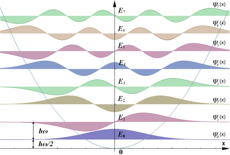
Fig. 2.1 Harmonic Oscillator with states \(\Psi = \{\psi_0, \psi_1, \psi_2, \dots, \psi_N\}\) and associated energies \(E = \{\epsilon_0, \epsilon_1, \epsilon_2, \dots, \epsilon_N\}\) CC by SA 3.0 Leyo, Tomasz59.